Lesson 3: Ohm’s Law
Table of Contents
- Ohm’s Law
- Make sure to use base units
- Let’s analyze some circuits!
- Activity: Using a circuit simulator
- Lesson summary
- Resources
- Next Lesson
In this lesson, we will learn about Ohm’s Law, one of the most important empirical laws in electrical circuits that describes how current, voltage, and resistance relate together. While Ohm’s Law is incredibly useful in analyzing and understanding how circuits work, like many “laws”, it is not always obeyed (particularly for what are called “non-ohmic” devices like LEDs or other diodes—which we will explore in Lesson 6: LEDs).
For now, on to Georg Ohm’s Law!
Ohm’s Law
In 1827, after years of experimentation, German physicist Georg Simon Ohm published the “Galvanic Circuit Investigated Mathematically”, which became the foundation for Ohm’s Law. Ohm’s Law states that the current (\(I\) in amperes) through a conductor equals the applied voltage (\(V\) in volts) divided by the conductor’s resistance (\(R\) in ohms):
\[I = \frac{V}{R}\]Thus, if we double the voltage in our circuit—for example, by stacking two batteries together in series—then we will also double the current. Ohm’s Law has many implications for how we build and use circuits with microcontrollers, including voltage dividers and resistive sensors.
Importantly, you will see and use Ohm’s Law in all three equivalent incarnations (which can be derived with simple algebra):
When you want to solve for current in your circuit, you use: \(I = \frac{V}{R}\)
To solve for voltage, use: \(V = I * R\)
To solve for resistance, use: \(R = \frac{V}{I}\)
Notice how these equations map to the concepts we explained in our first lesson on Voltage, Current, and Resistance—which you may want to return to. For example, \(I = \frac{V}{R}\) clearly demonstrates that to increase current, we can either increase voltage or decrease resistance.
Relating Ohm’s Law to our water analogies
Drawing again on our hydraulic-electric analogies (which we used amply in previous lessons), we can highlight another similarity. In the 1840s, Poiseuille empirically showed that the flow rate of water through a pipe is equal to the pressure drop across the pipe divided by the pipe’s resistance—this is called Poiseuille’s Law. And it conceptually makes sense: a higher pressure difference between two ends of a pipe creates more force and a lower resistance allows more water flow.
Does this equation sound familiar? It should. It is exactly Ohm’s Law! Current flow in a circuit is directly proportional to the voltage drop in a circuit divided by its resistance. See image below.
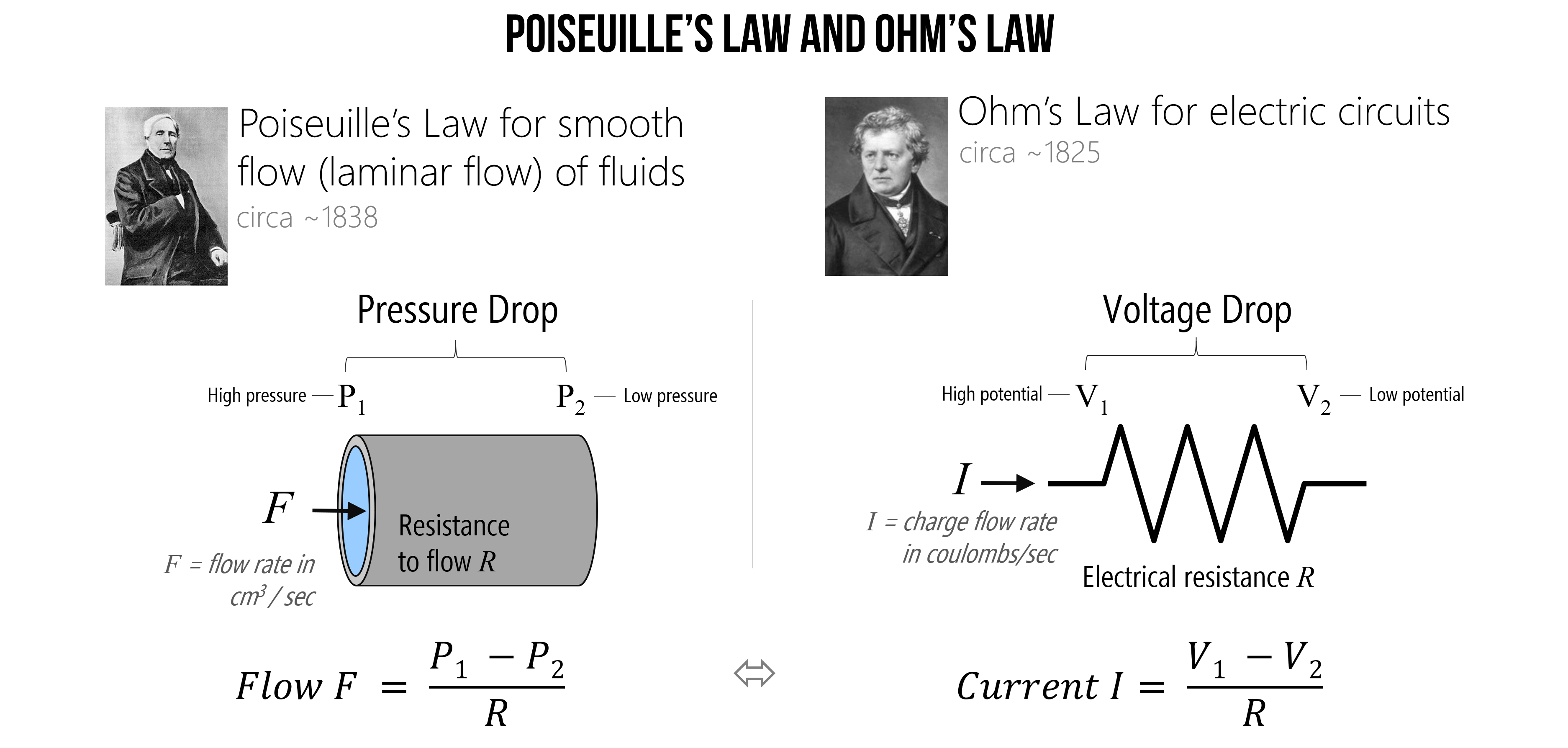
Figure. Poiseuille’s Law for the smooth flow of fluids and Ohm’s Law for electric current are similar. Image based on HyperPhysics at Georgia State and created in PowerPoint. Images of Poiseuille and Ohm are from Wikipedia.
Poiseuille’s Law equation only holds for the smooth (laminar rather than turbulent) flow of a Newtonian fluid like water. But such a stipulation is not relevant to electrical current.
Why \(I\) and not \(C\)?
You might be asking, “If \(R\) is the resistance in ohms (Ω) and V is the voltage in volts (V) then why is \(I\) used to represent the current in amperes (A) rather than \(C\)?” Two reasons: first, \(C\) is already reserved for the SI unit of coulombs (C), which is used in the very definition of amperes (recall that \(1\ A = 1\ C / s\)) and thus, could get confusing! Second, the ampere is named after André-Marie Ampère, considered the father of electromagnetism, who referred to amperage as the “intensité du courant” or “intensity of current.” So, current is \(I\) and not \(C\).
Make sure to use base units
A common “gotcha” in applying Ohm’s Law—or analyzing circuits in general—is messing up base units. In digital circuits, we often deal with kilohms (kΩ)—which is 1,000 ohms—milliamps (mA)—which is \(\frac{1}{1000}\) (0.001) of an amp—or even microamps (μA)—which is one millionth (\(\frac{1}{1,000,000}\) or 0.000001) of an amp—and so on. We need to convert these units to base units in volts (V), ohms (Ω), and amps (A) to perform our analysis.
For example, if a circuit contains a 2.2kΩ resistor with a 9V battery, to calculate the current do not mistakenly write \(I = \frac{9V}{2.2Ω}A\) but, instead, \(I = \frac{9V}{2200Ω}A\). The former would give you 4.1A (a large amperage and incorrect!) while the latter gives you the correct value of 0.0041A—which is 4.1mA.
So, always make sure you double check your units!
Common SI prefixes
Below, we’ve written some common SI prefixes—most of which should be familiar to you from other measurement quantities.
| Conversion factor | Scientific notation | Prefix | Abbreviation | English word | Examples |
|---|---|---|---|---|---|
| 1,000,000,000,000 | \(10^{12}\) | tera | T | trillion | terabyte, terameter |
| 1,000,000,000 | \(10^{9}\) | giga | G | billion | gigabyte, gigawatt |
| 1,000,000 | \(10^{6}\) | mega | M | million | megabyte, mega-awesome |
| 1,000 | \(10^{3}\) | kilo | k | thousand | kilobyte, kilometer, kilohm |
| 1 | \(1\) | base unit | gram, meter, amp, volt, ohm | ||
| 0.001 | \(10^{-3}\) | milli | m | thousandth | millimeter, milliamp, millivolt |
| 0.000001 | \(10^{-6}\) | micro | μ | millionth | micrometer, microamp |
| 0.000000001 | \(10^{-9}\) | nano | n | billionth | nanosecond, nanoamp |
| 0.000000000001 | \(10^{-12}\) | pico | p | trillionth | picosecond, picoamp |
Table. This chart is based on NIST’s Metric SI Prefixes webpage and Figure 2.2 in Bartlett’s book.
Converting units
To convert from a prefixed unit to a base unit, multiply by the conversion factor. To convert from a base unit to a prefixed unit, divide by the conversion factor.
So, for example, to convert 2.2kΩ to ohms, we would multiply by the conversion factor for kilo (k), which is 1,000. So, \(2.2 * 1,000 = 2,200 Ω\). To convert 0.000037A to microamps, we would divide by the conversion factor for micro (μ), which is 0.000001 (or \(10^{-6}\)). So, \(\frac{0.000037}{10^{-6}} = 37 μA\).
Let’s analyze some circuits!
Whew, OK, now we are ready to start analyzing some circuits. We’ll start with a simple circuit and go from there. When analyzing (or even preparing to build) circuits, it’s always a good idea to get out a pencil and paper. So, please do that now.
In addition, it’s helpful to have a way to check our work, which we can do in a circuit simulator. I like to use CircuitJS but I have also used EveryCircuit and CircuitLab—the latter costs money.
Before we begin, let’s watch this video of me building a simple resistive circuit in CircuitJS and calculating its current, given a voltage source and resistor.
Video. The video was created using the CircuitJS simulator. Direct link is here.
Example 1: Solve for current
Imagine a battery-powered circuit with a single resistor (basic, yes but pedagogically powerful!). If we are given the voltage \(9V\) and the resistance (\(100Ω\)), can we solve for the current \(I\)?
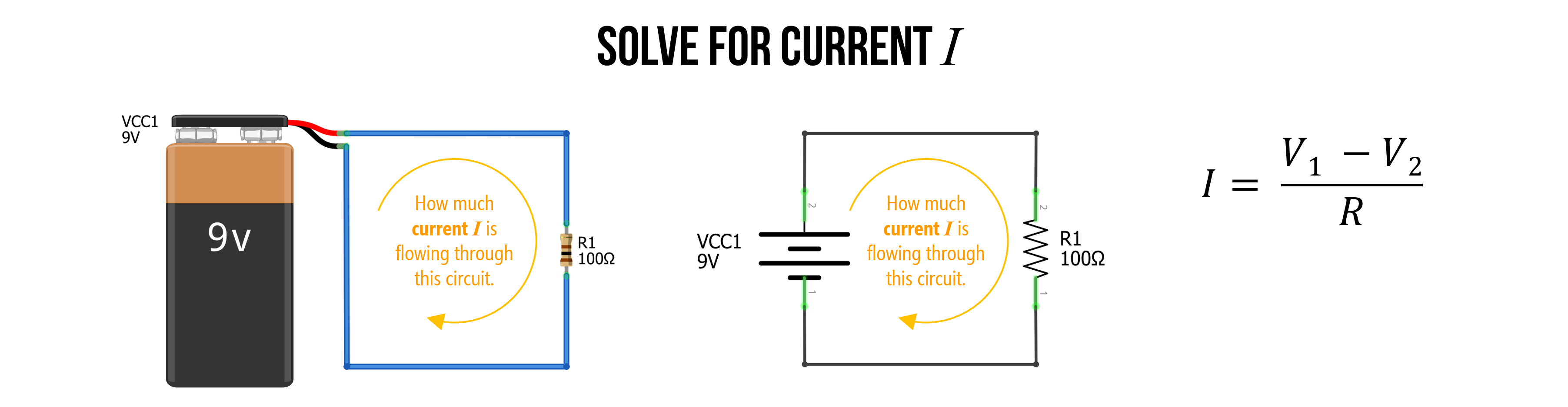
Figure. A simple 9V-powered circuit with a single resistor of \(100Ω\). Using Ohm’s Law, can you solve for current \(I\)? Images made in Fritzing and PowerPoint.
Step 1: Identify knowns
To begin your analysis, you’ll want to identify everything that you know about this circuit.
Observe that all wires touching the positive battery terminal have the same electric potential (\(9V\))—which we’ve now marked in red—and all wires touching the negative battery terminal have the same electric potential (\(0V\))—which we’ve marked in black. Note that even though copper wires have some resistance, it’s so small (especially for the lengths in a digital circuit), that we can model it as \(0Ω\) (indeed, wires are always assumed \(0Ω\) in this sort of circuit analysis).
And because we are solving for current, we need to use the Ohm’s Law formulation: \(I = \frac{V}{R}\). More specifically, as voltage is always relative—an electric potential difference—we use \(I = \frac{V_1 - V_2}{R}\)

Figure. All wires touching the battery’s positive terminal have the same voltage (9V). Similarly, all wires touching the battery’s negative terminal have the same voltage (0V). Images made in Fritzing and PowerPoint.
Step 2: Apply knowns
Having established that all of the wires on the top of the circuit (those directly connected to the positive terminal) are the same electric potential, we can mark it as a single node \(V_1\). Similarly, all wires touching the negative battery terminal can be called node \(V_2\).
Now, we can substitute \(9V\) for \(V_1\) and \(0V\) for \(V_2\). And we also know that \(R=100Ω\), giving us the complete equation: \(I = \frac{9V - 0V}{100Ω}\)
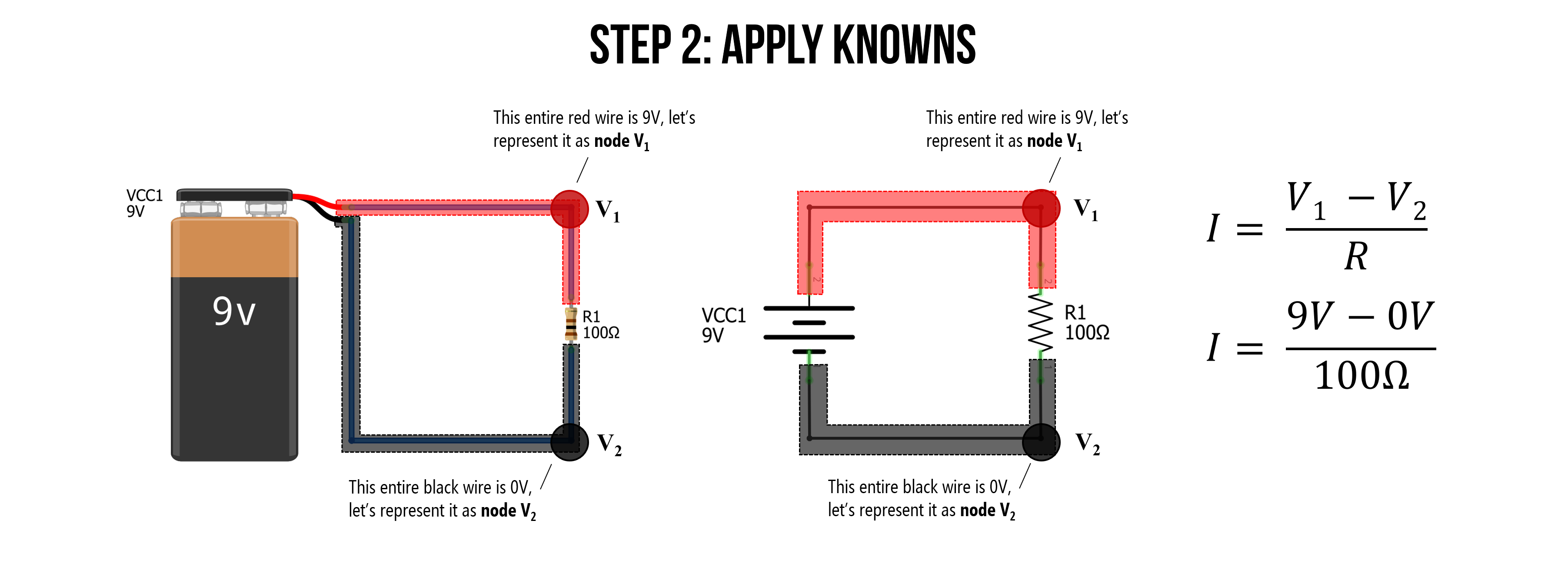
Figure. We can call all wires touching the battery’s positive terminal node \(V_1\) and all wires touching the negative terminal node \(V_2\). Using this information, we can substitute \(9V\) for \(V_1\) and \(0V\) for \(V_2\). Images made in Fritzing and PowerPoint.
Step 3: Solve for current I
Finally, we are ready to solve for current \(I = \frac{9V - 0V}{100Ω} \Rightarrow 0.09A \Rightarrow 90mA\)
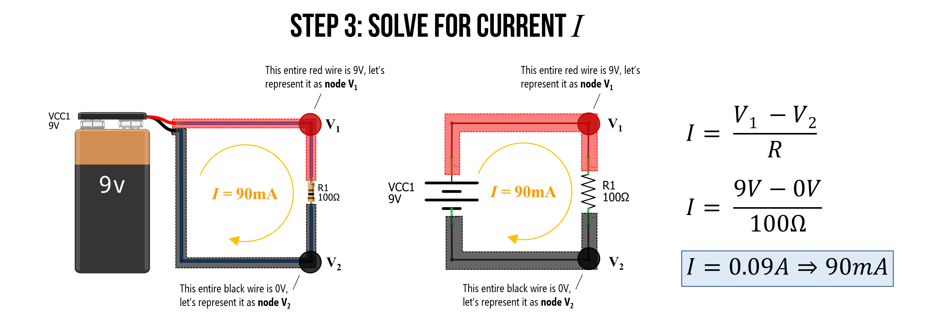
Figure. We successfully applied Ohm’s Law to solve for current: \(I = 90mA\).
Example 2: Solve for current again (but with different resistance)
Let’s try to solve for current again with a similar circuit. This time the resistance has been increased from \(100Ω\) to \(4.7kΩ\).
Before doing anything else, it’s useful to think conceptually about what will happen.
Current decreases, right? And does so proportionally.
Indeed, the current goes from \(90mA\) with \(100Ω\) to \(I = \frac{9V}{4700Ω} \Rightarrow 0.0019𝐴 \Rightarrow 1.9𝑚𝐴\), which is not very much!
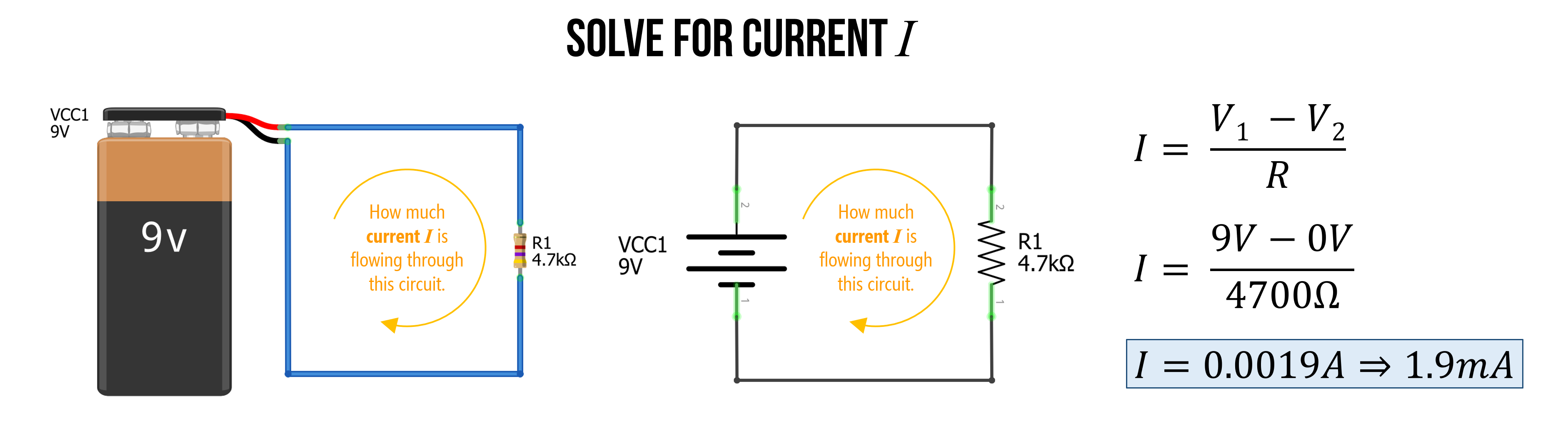
Figure. As expected, the current \(I\) goes down as resistance \(R\) goes up.
Example 3: Solve for voltage
As noted above, we can use the three different formulations of Ohm’s Law (\(I=\frac{V}{R}\), \(V=I*R\), and \(R=\frac{V}{I}\)) to help us analyze different unknowns in a circuit.
In this case, let’s use Ohm’s Law to solve for an unknown voltage source. Assume a similar circuit as before: a single voltage source (but of unknown voltage) with a single resistor of size \(100Ω\) and a current of \(I=50mA\).
Because we are solving for voltage, we should use the \(V=I*R\) formulation. The first thing we need to do is ensure that all of our measurements are in base units. The current is not, so modify it to amperage (rather than milliamps): \(I=50mA \Rightarrow 0.05A\).
Now, we can easily solve for \(V = 0.05A * 100Ω = 5V\). The battery is a \(5V\) voltage source.
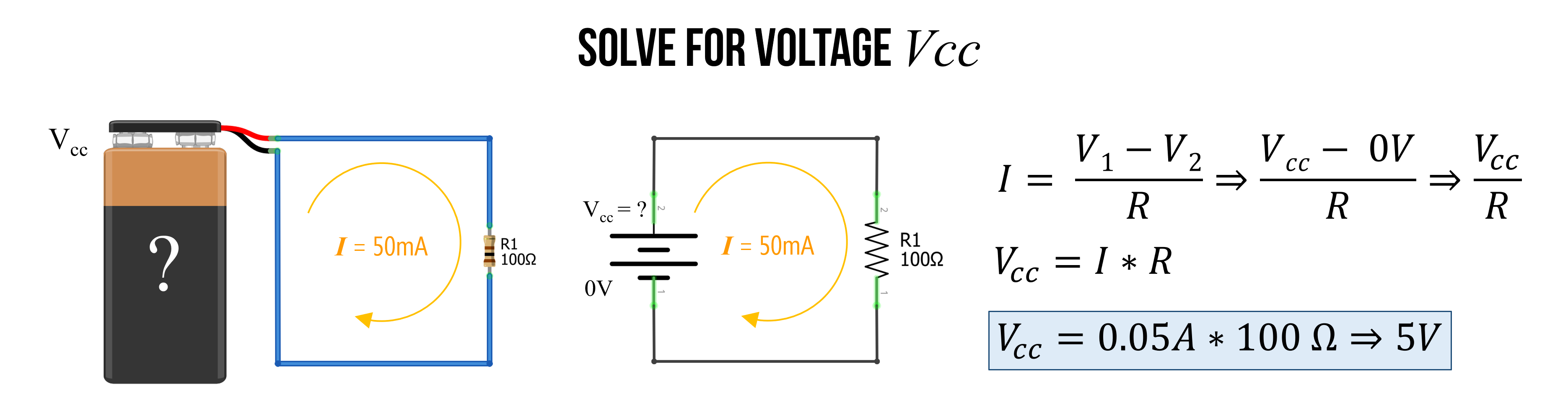
Figure. Using the \(V=I*R\) formulation of Ohm’s Law, we can solve for voltage given a known current \(I\) and a known resistance \(R\). Images made in Fritzing and PowerPoint.
Example 4: Solve for resistance
I bet you’re getting the hang of it now!
Finally, you can use \(R=\frac{V}{I}\) to solve for resistance if \(V\) and \(I\) are known. In this case, let’s return to our \(9V\) battery and assume we have a current of \(1.32mA\). What is the resistor value \(R\)?
Again, the first thing to do is convert all units to base units. So, \(1.32mA \Rightarrow 0.00132A\).
Now, we can solve for \(R = \frac{9V}{0.00132A} \Rightarrow 6818.2Ω \Rightarrow 6.8kΩ\)
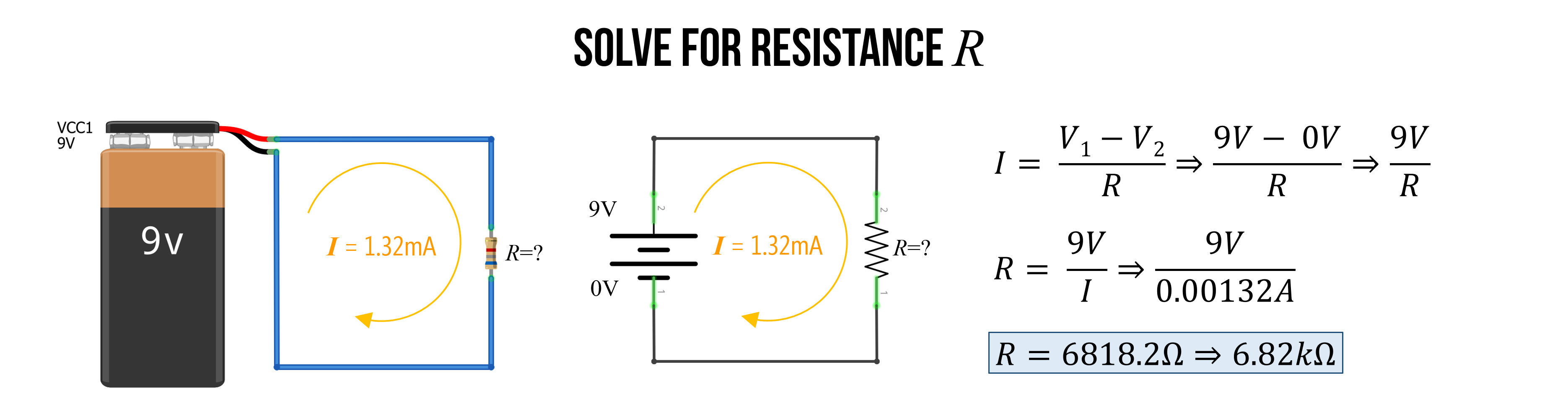
Figure. Using the \(R=\frac{V}{I}\) formulation of Ohm’s Law, we can solve for the resistance \(R\) given a known voltage \(V\) and a known current \(I\). Images made in Fritzing and PowerPoint.
Try it yourself
Before moving on to the activity, try solving these three problems on your own. Check your work using the formulas above—and pay attention to units!
- A circuit has a 5V battery and a 1kΩ resistor. What is the current?
- A circuit draws 15mA of current through a 330Ω resistor. What is the voltage drop across the resistor?
- A 9V battery produces 4.5mA of current in a circuit with a single resistor. What is the resistance?
Answers. (1) \(I = \frac{5V}{1000Ω} = 5mA\). (2) \(V = 0.015A \times 330Ω = 4.95V\). (3) \(R = \frac{9V}{0.0045A} = 2000Ω = 2kΩ\).
Activity: Using a circuit simulator
Now that we’ve built up an initial understanding of Ohm’s Law, it’s time to build and play with some circuits in a circuit simulator.
Using CircuitJS, build and analyze five different types of resistive circuits. You can build whatever circuits you want with a few requirements:
- All circuits should have only a single power supply
- You should use only resistors
- You can use as many resistors per circuit as you’d like but double click on the wires to show current/voltage
- For each circuit, take a screenshot and put it in your prototyping journal along with a brief reflection of what you observed/learned.
You can save your circuits in one of two ways: (1) download them locally (File -> Save As) or (2) export them as a shareable link (File -> Export as Link)—use this latter option for your prototyping journals.
In your prototyping journals, include a screenshot of each CircuitJS circuit along with a brief description of what you observed and a link directly back to the CircuitJS circuit that you made.
Lesson summary
In this lesson, we learned:
- Ohm’s Law is an empirical law that describes the linear relationship between voltage, current, and resistance: \(I = \frac{V}{R}\)
- This law builds on the concepts and intuitions we developed in Lesson 1, and can be rearranged to solve for any one of the three quantities given the other two
- A common “gotcha” for beginners is forgetting to convert measurements to base units (volts, amps, ohms) before applying Ohm’s Law
- We applied Ohm’s Law to simple single-resistor circuits and verified our calculations using CircuitJS
Resources
-
Introduction to Ohm’s Law, Khan Academy
-
What is Ohm’s Law?, Math and Science
Next Lesson
In the next lesson, we will apply Ohm’s Law to more complex circuits—specifically those that combine resistors in series and those that combine them in parallel.