Sensors
Table of Contents
- Passive vs. active sensing
- Sensor output
- Evaluating a sensor
- Signal acquisition pipeline
- Let’s make stuff!
From an early age, we are taught of the five basic human senses: touch, sight, hearing, smell, and taste. But we don’t often think about just how sophisticated and wonderfully complex the human sensing system is from our largest organ, our skin, which can sense temperature and various tactile stimuli (pressure, texture, vibration) to our eyes and optic nerves, which can dynamically focus, adapt to lighting levels, and even help preattentively identify moving objects and other shapes. And this interconnected network of sensors function in real-time, transmitting information to the brain for processing and analysis. Amazing!
Still, we can’t sense everything. Dolphins and bats use echolocation to navigate and forage using high-frequency sound pulses, some fish use electrolocation to navigate murky waters by generating electric fields and detecting distortions in these fields using electroreceptor organs, some snakes have infrared vision allowing them to see at night, and other animals have the ability to sense and detect a magnetic field to perceive direction, altitude, or location (called magnetoreception).
Even for the senses that we do have—as remarkable as they are—our senses will never be as precise or refined as a hawk’s vision, a wolf’s smell, or a cat’s hearing. And, even then, there are far more things to sense in the world than there are biological sensors.
For computing, sensors provide a way to access information about the world, human activity, and beyond. And electronic sensors are not limited to biology—as amazing and diverse as it is—but rather to our own ingenuity in coming up with ways to capture the world. This is an incredibly exciting challenge!
With advances in sensing technology like MEMs, computing (storage, networking, wearables), and in processing and machine learning, now is a fascinating time to think about and study the role of sensing in an increasingly computational society.
How can new sensing and processing systems help identify cancer cells, find new life-supporting planets, or change how we fundamentally interact with computing itself (ala capacitive touchscreens on tablets and phones!)?
In addition to what a sensor does, we can characterize them by how they sense and what output they provide.
Passive vs. active sensing
There are two basic classes of sensors: active and passive. Active sensors require external power (and will thus have a Vcc pin and GND) while passive sensors do not. Yes, that’s it. That’s the key difference! For example, the popular ADXL335 3-axis accelerometer is an active sensor: it has a Vin, a GND, and three analog outputs (Xout, Yout, and Zout), which translate acceleration along each axis into ratiometric (proportional) voltage levels. In contrast, a thermistor is a passive sensor: it changes its resistance in response to heat, which can be used to calculate temperature.
Some active sensors transmit a signal and then analyze some reflected property of that signal for sensing. For example, an infrared (IR) proximity sensor like the Sharp GP2Y0A21YK contains both an infrared (IR) transmitter and IR receiver. The sensor calculates distance by transmitting an IR beam and measuring the reflection angle back on the IR receiver. Similarly, an ultrasonic distance sensor like the popular HC-SR04 transmits ultrasonic pings and listens for reflected ultrasonic waves. A connected microcontroller can than calculate the distance between the sensor to the sound-reflecting object by using the speed of sound through air.
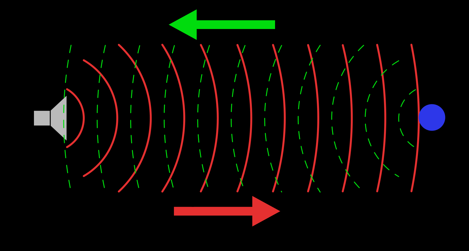 Ultrasonic distance sensors are a type of active sensor consisting of both a transmitter and receiver. They work by transmitting an ultrasonic pulse, which is partially reflected back by objects in the sound wave path (if any). By measuring the time between the pulse transmission and the echo reception, distance can be determined.
Active sensors may also include sophisticated (but tiny) on-board hardware to counteract sensor drift, to filter/smooth a signal, and/or to communicate output via a digital communication protocol like I2C.
In contrast, a passive sensor generates an output signal based on some external stimulus and does not require external power. For example, a photoresistor changes its resistance in response to light, a thermistor in response to temperature, and a force-sensitive resistor in response to pressure. Of course, we need a powered circuit to “retrieve” information from the sensor—like a voltage divider—but the underlying sensor is responding to environmental phenomena regardless of this applied power.
A simple heuristic to distinguish active from passive sensors is to count pins: active sensors have at least three pins (one for Vin, one for GND, and at least one for output) while passive sensors have two.
Sensor output
Sensors output either analog, binary (on/off), or digital signals (e.g., SPI). Yes, “binary” is a type of digital output but it’s worth distinguishing.
Analog output
Pure analog sensors include resistive sensors, like the aforementioned thermistors and photoresistors, which change their resistance based on some stimuli as well as ratiometric sensors like the aforementioned ADXL335 accelerometer or the DRV5055 Hall Effect sensor, both which vary their voltage output linearly in response to some stimuli—in this case, acceleration and magnetic fields, respectively.
Digital output
Many modern sensors are chip-based and include some on-board processing. These sensors process and convert raw analog signals to digital output. This output is stored in a memory location (called a register) on the sensor chip itself and accessed by a microcontroller via a communication protocol like I2C and SPI.
For example, in contrast to the ADXL335 accelerometer, which outputs a voltage proportional to acceleration on each axis on pins X, Y, and Z, the LIS3DH accelerometer communicates over either I2C or SPI. We often supply one or the other in our hardware kits.
Because the LIS3DH supports a digital communication protocol (both I2C and SPI), you can configure the sensor hardware via code (e.g., set the acceleration range from +-2g to +-16g). This is a nice benefit of sensors with built-in chips but can also increase their cost.
| ADXL335 Accelerometer | LIS3DH Accelerometer |
|---|---|
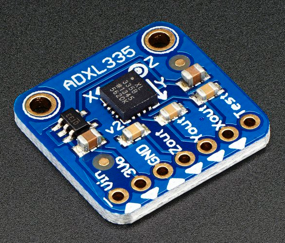 | 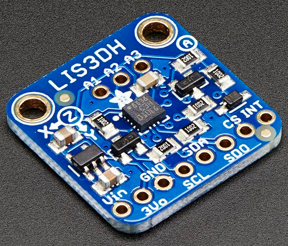 |
Binary output
Finally, some “sensors” are either on or off (which could be construed as a type of simple digital output but not one specifically encoded for a microcontroller so does not qualify as “digital signal” in our taxonomy). For example, reed switches close in the presence of a magnetic field and tilt ball switches are hollow tubes with an enclosed conductive ball, which moves to close internal contacts in certain tube orientations (or tilts).
Platt provides an even deeper breakdown of sensor output types, including open collectors and sensors that change in current rather than voltage. See his book for details.
Evaluating a sensor
There are a variety of important criteria when evaluating a sensor’s capabilities, including:
- Sampling rate: How fast does the sensor provide output?
- Resolution: What is the smallest change in physical quantity that the sensor can identify?
- Quantization error: What is the error caused by rounding due to digitizing the analog data in the ADC? See Signal acquisition pipeline section below.
- Absolute error: What’s the difference between sensor readings and the true physical quantity?
- Drift: How does the absolute error change over time while operating the sensor?
- Environmental stability: How does the sensor change in response to differences in temperature or moisture?
Signal acquisition pipeline
Let’s examine the entire signal acquisition pipeline from raw physical signal to the digitized representation. We’ll learn more about signals and signal processing in the Signals lessons.
- First, there exists some physical phenomena that exists in the world (Stage 1).
- We need to develop and/or utilize a method to sense that phenomena and output an electrical signal (which will be readable by a computer) (Stage 2).
- Some sensor chips process this electrical signal (e.g., smooth, filter, amplify)—Stage 3.
- In Stage 4, an analog-to-digital converter (ADC) converts the electrical signal to bits (a process called quantization).
- Finally, in Stage 5, we can process and analyze the digitized signal using digital signal processing (DSP) techniques and machine learning, woohoo!
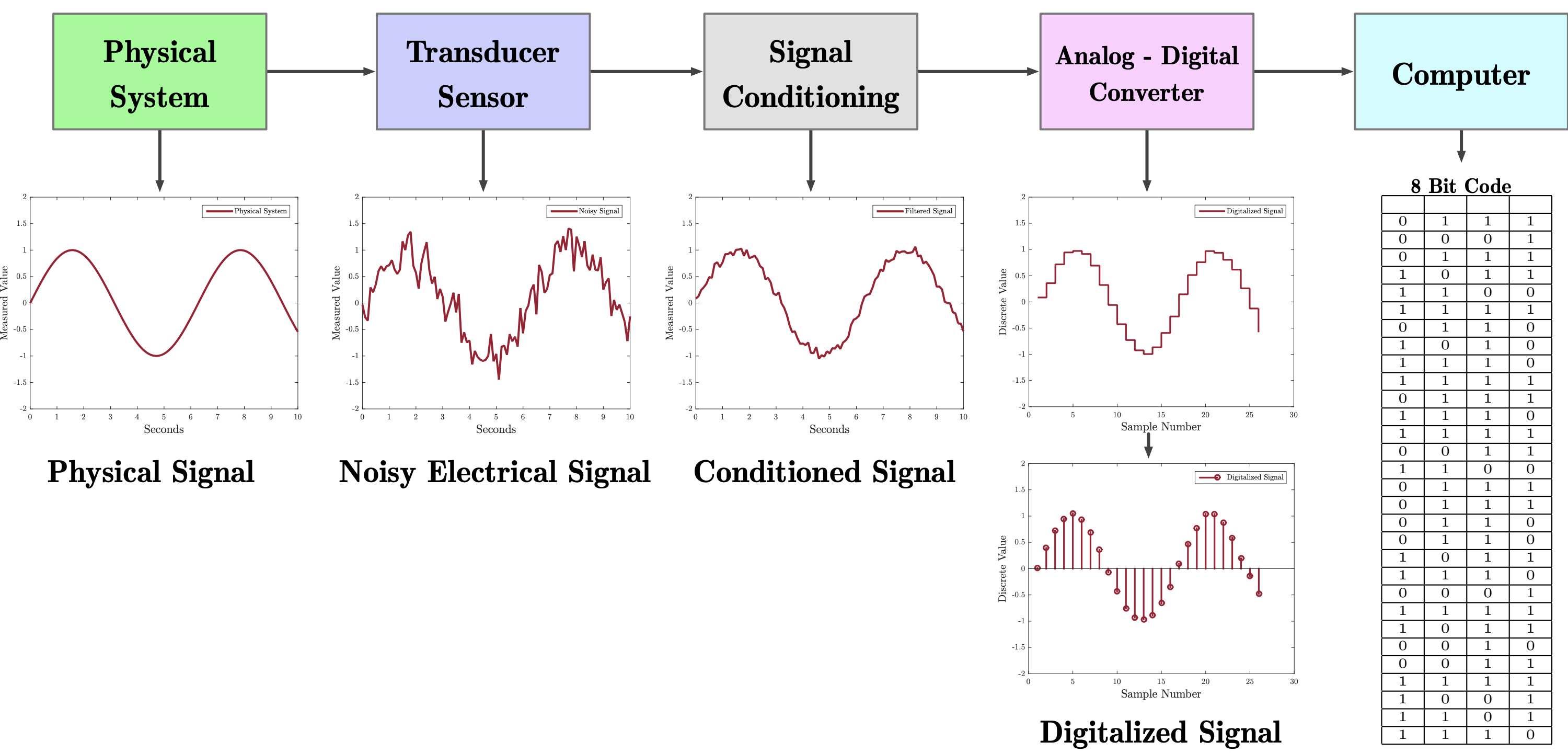 Block diagram from Wikipedia “Data acquisition” article. Direct link.
Some signal acquisition considerations
When selecting sensors and a data processing pipeline, there are multiple considerations, including:
- Sampling rates. How often does the target physical signal change? How quickly can your sensor respond? Does this response rate matter? A photoresistor, for example, takes several milliseconds to respond to bright light and can require more than one second to regain its dark resistance while a phototransitor and photodiode are more responsive (see Platt).
- ADC conversion rates How fast can your microcontroller sample the signal and perform the analog-to-digital conversion?
- ADC precision What precision of ADC do you need? The ATmega328 microcontroller uses a 10-bit ADC. So, by default, the voltage range of 0-5V is mapped to 0-1023 \(2^10\) and, thus, the resolution between readings is 5V / 1024 or 0.0049 volts (4.9 mV). If you require greater precision—that is, changes in sensor output < 0.0049V are important—then you either need to change the
analogReferenceor you need a different ADC. The difference between a raw continuous signal and its digitized version is called the quantization error.
Nyquist sampling theorem
One of the most important (and interesting!) theorems in DSP is the Nyquist-Shannon Sampling Theorem, which states that a continuous time signal (the raw physical signal) can be sampled and perfectly reconstructed if the sampling rate (sometimes called the sampling frequency or \(F_s\)) is over twice as fast as the raw signal’s highest frequency component. That is, the minimum sampling frequency \(min(F_s)\) must be greater than \(2 * max(F_{signal})\).
For example, a common digital audio sampling rate is 44,100Hz (44.1 kHz). This is what compact discs (CDs) use and is also standard for mp3s. Why 44.1 kHz? This sampling rate was chosen, in part, because the human hearing range is ~20 Hz to 20kHz. Hence, according to the above theorem, the minimum sampling frequency needed to be at least \(2 * 20kHz\) or 40kHz.
To learn more about the Nyquist sampling theorem along with concrete, interactive examples, please see our Quantization and Sampling Jupyter Notebook.
ATmega328 ADC conversion rate
The ATmega328 ADC requires an input clock frequency between 50kHz and 200kHz (Section 24.4 of datasheet). A normal conversion takes 13 ADC clock cycles (though the very first conversion takes 25 ADC clock cycles to initialize the analog circuitry).
The ATmega328 CPU and ADC share the same clock; however, the microcontroller clock is too fast (16MHz) for the ADC, so you can control a “prescaler” to divide the CPU clock into an acceptable range (divisors are 2, 4, 8, 16, 32, 64, 128). By default, the Arduino library sets the prescaler to 128 (16MHz/128 = 125 KHz) in wiring.c (by setting a bit in a configuration register). Since a conversion takes 13 ADC clocks, the sample rate is about 125KHz/13 or 9600 Hz. And this doesn’t consider the overhead of the other code running on the microcontroller.
Is this fast enough? For a vast majority of human-oriented sensing, yes! For example, video games target 60 fps (60Hz) refresh rates and human reaction time is ~150-250 ms (~4 Hz). So, 9600Hz is blazingly fast in comparison! For sampling sound, however, 9600Hz is on the low end. Recall that most digital music files have a sampling rate of 44.1 kHz—4.6 times faster than the ATmega328’s 9600Hz. At 9600Hz, the maximum recognizable frequency in the sound wave would be 4800Hz. We’ll investigate this further in the Signals portion of the class.
Note: It is possible to sample the ATmega328 at a faster rate but at a cost of accuracy. The ATmega328 datasheet warns that if the ADC input clock frequency exceeds 200kHz then not all 10 bits of conversion may be ready (perhaps just the first 8 bits or less). If you want to learn more about faster analog reads on the Arduino, Open Music Labs has explored the speed/quality tradeoffs of the ATmega328 ADC here and here. In addition, this blog post talks about using the “ADC Free Running mode” with interrupts to get a 76.8 KHz sampling rate (and also links here).
ATmega328 ADC resolution
By default, the ADC resolution on the ATmega328 is 10bits (0-1023) across 0-5V. So, a 4.88mV resolution (smallest recognizable voltage step). You can change this, however, if you do not need the full 0-5V range.
Indeed, the Arduino library supports changing the ADC range from the default of \(0-5V\) to \(0-X\) where \(X\) is any value between 1.0V and \(V_{cc}\) (which is 5V on the Uno). You can do this via the analogReference function. This may be useful, for example, if you know that your sensors output voltage ranges between 0-3.3V, then setting analogReference(EXTERNAL) and applying 3.3V to the AREF pin on the Arduino improves the ADC resolution from 4.9mV to 3.2mV.
Tronixstuff.com has a nice AREF tutorial.
Let’s make stuff!
With that, let’s make some stuff with sensors!
The lessons below assume that you’ve completed both our Intro to Output and Intro to Input series.
Force
Learn how to sense force using a force-sensitive resistor (FSR). This is what you did in the Intro to Input series.
Light
Learn how to sense light using a photoresistor (aka photocell).
Magnetic fields
Learn how to sense magnetic fields using a Hall effect sensor.
Distance
Learn how to sense distance (2-400cm) using the HC-SR04 ultrasonic distance sensor
Sound
Learn how to sense sound using an electret microphone with a MAX4466 amplifier.
Accelerometer
Learn how to sense acceleration using the LIS3DH 3-axis accelerometer.