Signals
Table of Contents
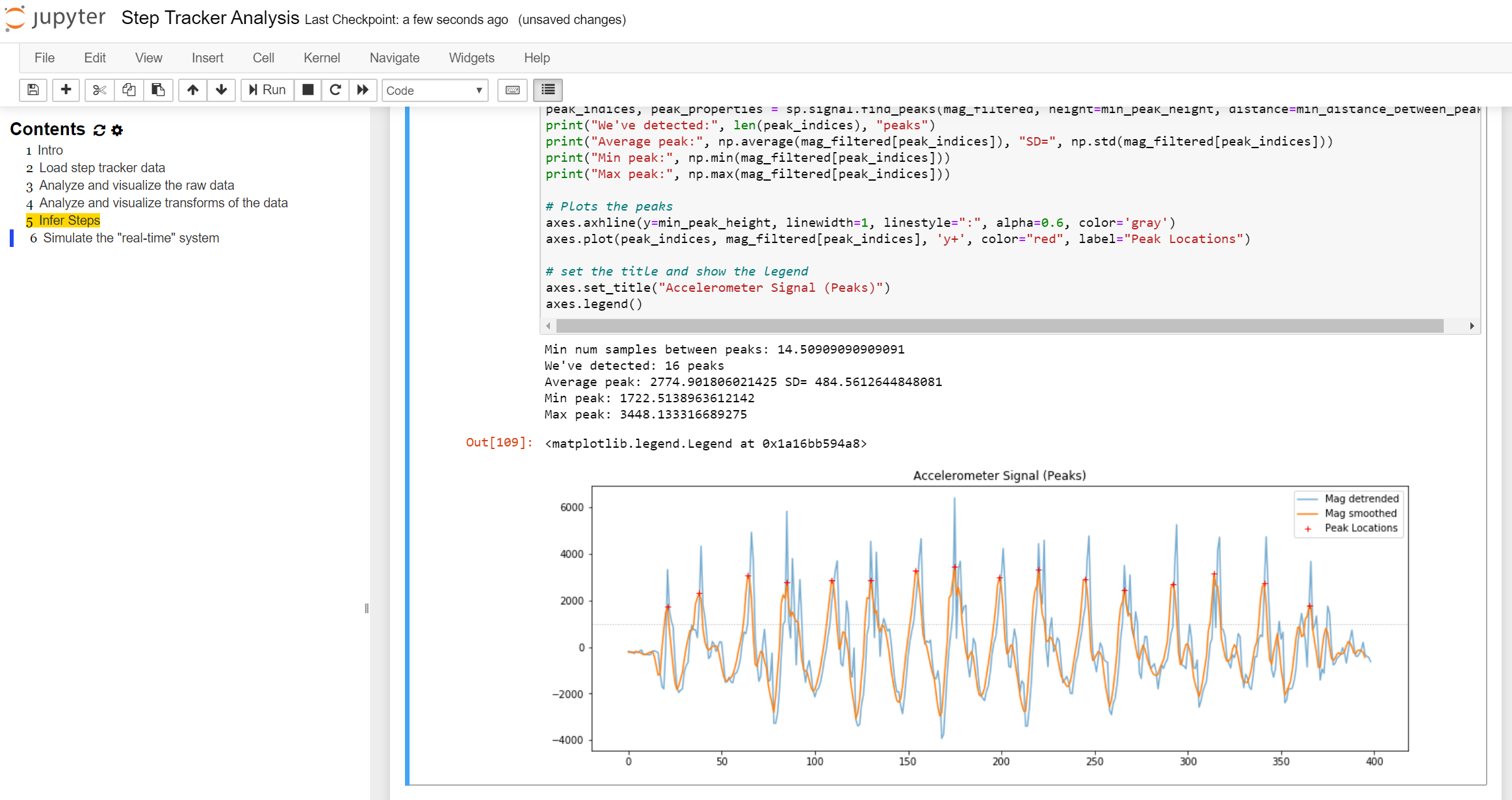
Jupyter Notebook screenshot showing an analysis and visualization of a 3-axis accelerometer to infer step counts.
We will be using Jupyter Notebook for the signal processing and machine learning portion of our course. Jupyter Notebook is a popular data science platform for analyzing, processing, classifying, modeling, and visualizing data. While Notebook supports multiple languages (like R, Julia), we’ll be using Python (specifically, Python 3). For those familiar with Python, Jupyter Notebook is built on the IPython kernel so you can use all of the IPython magic commands!
For analysis, we’ll be using the SciPy (“Sigh Pie”) ecosystem of open-source libraries for mathematics, science, and engineering. Specifically, NumPy, SciPy, and matplotlib. We may also dabble in Pandas and Seaborn. For machine learning, we’ll be using sci-kit learn. And don’t worry, all of these libraries will be managed and installed for us!
Just like for Arduino, there is a plethora of wonderful tutorials, forums, and videos about Jupyter Notebook and the SciPy libraries. Please feel free to search online and to share what you find with the class.
Lessons
These lessons are intended to be interactive. You should modify, run, iterate, and play with the cells. Make these notebooks your own!
There are three ways to view the lessons: first, you can click on the exported HTML versions; however, these are not interactive; second, you can clone our Signals repo and open the ipynb files locally on your computer (this is our recommended approach):
git clone https://github.com/makeabilitylab/signals.git
Third and finally, if you want a quick, easy method to interact with the notebooks, you can use Binder or Google Colab—both cloud services dynamically load our notebooks directly from GitHub, so you can play, edit code, etc. right from your browser—and just a click away. Yay!
Note: Again, for your actual assignments, you’ll likely want to run your notebooks locally because you’ll want to load data from disk. You can also do this with Google Colab (you’ll just need to get your data into the cloud environment; see below).
Introduction to Jupyter Notebook, Python, and SciPy
Lesson 0: Install Jupyter Notebook and Tips
In our initial lesson, we will learn how to install Jupyter Notebook, a helpful extension that auto-generates table of contents, and go over some tips.
Lesson 1: Introduction to Jupyter Notebook
There are many introductory tutorials and videos to Jupyter Notebook online. We’ll quickly demo Notebook in class but if you want to learn more, you could consult this Datacamp tutorial or this Dataquest tutorial. Regardless, you will learn Notebook as you go through the lessons below and work on your assignments.
Lesson 2: Introduction to Python (ipynb)
If you’re not familiar with Python—or even if you are—it’s a good idea to start with this (rapid) introduction to Python. It will also give you a feel for Jupyter Notebook. To gain the most value from these example Notebooks, you should modify and run the cells yourself (and add your own cells). ![]()
![]() .
.
Lesson 3: Introduction to NumPy (ipynb)
We’ll be using NumPy arrays as one of our primary data structures. Use this notebook to build up some initial familiarity. You need not become an expert here but it’s useful to understand what np.array’s are and how they’re used and manipulated. ![]()
![]()
Lesson 4: Introduction to Matplotlib (ipynb)
For visualizing our data, we’ll be using Matplotlib—an incredibly powerful visualization library with a bit of an eccentric API (thanks to Matlab). Open this notebook, learn about creating basic charts, and try to build some of your own. ![]()
![]()
Signals
Lesson 1: Quantization and Sampling (ipynb)
Introduces the two primary factors in digitizing an analog signal: quantization and sampling. Describes and shows the effect of different quantization levels and sampling rates on real signals (audio data) and introduces the Nyquist sampling theorem, aliasing, and some frequency plots.
Lesson 2: Comparing Signals (Time Domain) (ipynb)
Introduces techniques to compare signals in the time domain, including Euclidean distance, cross-correlation, and Dynamic Time Warping (DTW).
Lesson 3: Frequency Analysis (ipynb)
Introduces frequency analysis, including Discrete Fourier Transforms (DFTs) and the intuition for how they work, Fast Fourier Transforms and spectral frequency plots, and Short-time Fourier Transforms (STFTs) and spectrograms.
Exercises
Exercise 1: Step Tracker (ipynb)
Building off our A2 assignment, let’s analyze some example accelerometer step data and write an algorithm in Jupyter Notebook to infer steps. Notebook is perfectly suited for this task: it’s easy to visualize data with Matplotlib and NumPy and SciPy offer filtering, detrending, and other useful signal processing algorithms. You can try lots of ideas, see how well they work on some test data, and then implement your most promising idea on the ESP32. ![]() .
.
Exercise 2: Gesture Recognizer: Shape Matching (ipynb)
Let’s build a shape-based (or template-based) gesture recognizer! This Notebook provides the data structures and experimental scaffolding to write and test shape-based gesture classifiers.
Exercise 3: Gesture Recognizer: Supervised Learning (ipynb)
Let’s build a feature-based (or model-based) gesture recognizer using supervised learning! This Notebook provides an overview of how to use supervised learning and the Scikit-learn library to classify gestures.
Exercise 4: Gesture Recognizer: Automatic Feature Selection and Hyperparameter Tuning (ipynb)
In this Notebook, you’ll learn about automatic feature selection and hyperparameter tuning.